Calculating Confidence Interval in R
Confidence intervals (CI) are part of inferential statistics that help in making inference about a population from a sample. Based on the confidence level, a true population mean is likely covered by a range of values called confidence interval. A basic rule to remember, the higher the confidence level is, the wider the interval would be. Whenever CI are reported, it is essential to focus on the reported confidence level.
The figure below shows a 95% confidence interval of a normal distribution:
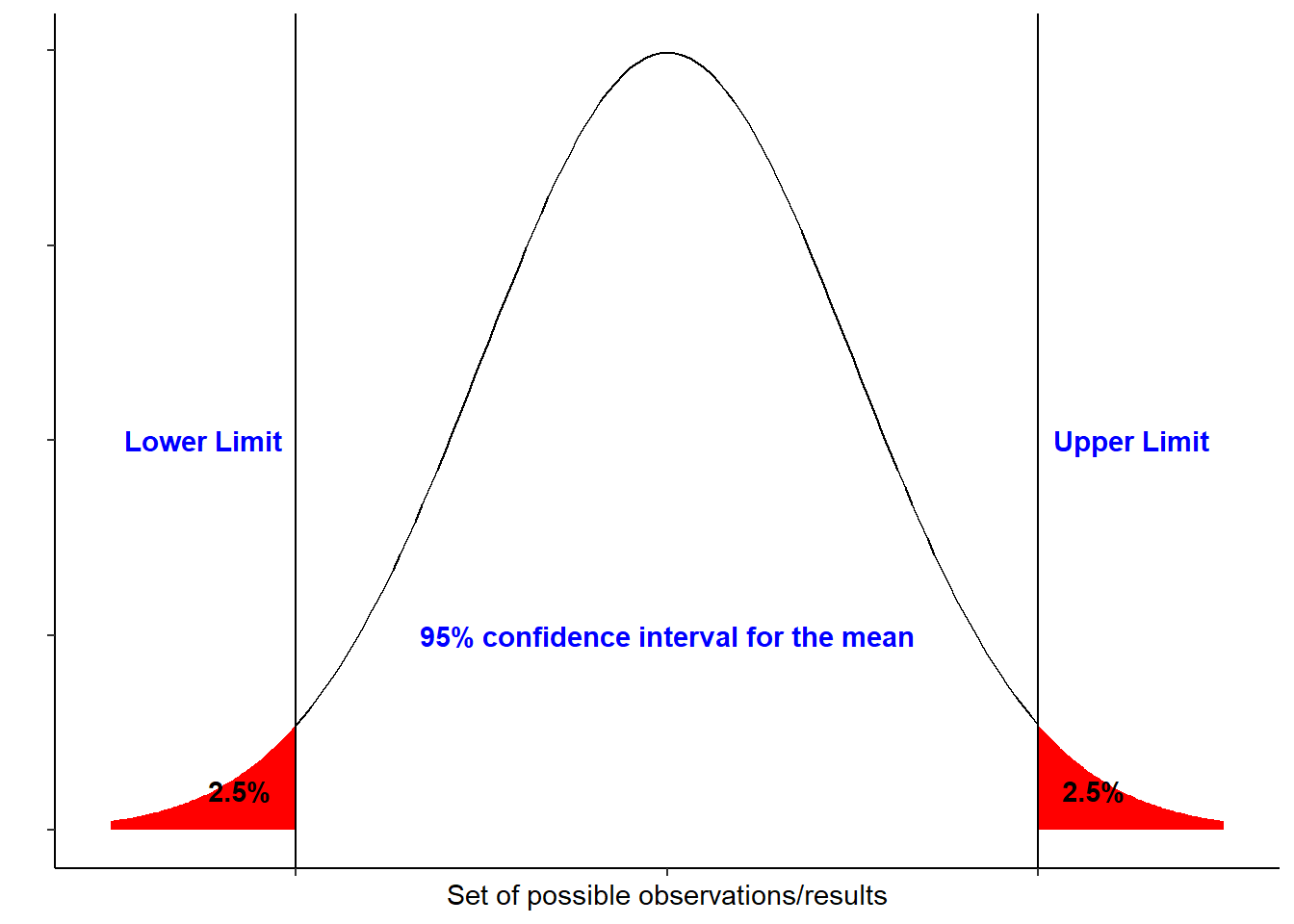
If we repeat an experiment/sampling method 100 times, 95% of the times would include the true population mean. Basically the larger the sample size the narrower the interval would be.
The basic information needed to calculate the CI are the sample size, mean and the standard deviation. These values resemble a descriptive measure of the sample/cohort.
Sample size/number of samples: \(n\)
Average mean \[\bar{X} = \frac{\sum_{} x_{i}}{n}\]
Standard deviation \[s^{} = \sqrt{\frac{\sum (x_{i} - \bar{X})^{2}}{n - 1}}\]
CI using t-tables or z-tables:
- The CI formula when the experimental design/sample sizes are small or when the standard deviation of the population is unknown:
\[\mathrm{CI} = \bar{X} \pm (t_{n - 1} \times\frac{s}{\sqrt{n}})\] The \(t_{n-1}\) is taken from the \(t\) distribution based the degree of freedom and on the probability \(\alpha\) that CI does not include the true population mean.
- When the experimental design/sample sizes are large or when the standard deviation of the population is known then CI formula is:
\[\mathrm{CI} = \bar{X} \pm (z_{\frac{1 - α}{2}} \times\frac{s}{\sqrt{n}})\] The \(z_{\frac{1 - \alpha}{2}}\) is taken from the \(z\) distribution based on the probability \(\alpha\) of the confidence level. Since \(\alpha\) is the probability of confidence interval not including the true population parameter, thus 1 - \(\alpha\) is equal to the probability that the population parameter will be included in the interval.
Example: Assume Scientists came up with a vaccine against a certain virus and are 95% confident that mean antibody titer production induced by the vaccine is 15 IU/L. To test their hypothesis a clinical trial was conducted. The vaccine was administered to 25 subject/patients, after a specific period, the anitbody titer in the blood was measured for each patient. The measurements of the vaccinated patients are shown below:
##  [1] 15.40  9.21  4.20  7.50 12.20 18.30 17.30 14.30 14.02 20.00 12.30 14.10
## [13] 17.30 15.40 12.20 11.40  9.10 18.00 14.43 17.00 15.10 13.40 15.30 12.20
## [25] 13.30
The mean antibody titer of the sample is 13.72 and standard deviation is 3.6. By applying the CI formula above, the 95% Confidence Interval would be [12.23, 15.21]. This indicates that at the 95% confidence level, the true mean of antibody titer production is likely to be between 12.23 and 15.21. However there is a 5% chance it won’t.
The function below computes the CI based on the \(t\) distribution, it returns a data frame containing descriptive measures and the CI.
CI_t <-  function (x, ci = 0.95)
{
  `%>%` <- magrittr::`%>%`
  Margin_Error <- qt(ci + (1 - ci)/2, df = length(x) - 1) * sd(x)/sqrt(length(x))
  df_out <- data.frame(  sample_size=length(x), Mean=mean(x), sd=sd(x),
                         Margin_Error=Margin_Error,
                         'CI lower limit'=(mean(x) - Margin_Error),
                         'CI Upper limit'=(mean(x) + Margin_Error)) %>%
    tidyr::pivot_longer(names_to = "Measurements", values_to ="values", 1:6 )

  return(df_out)
}
The function below computes the CI based on the \(z\) distribution, it also returns a data frame containing descriptive measures and the CI.
CI_z <-  function (x, ci = 0.95)
{
  `%>%` <- magrittr::`%>%`
  Margin_Error <-  abs(qnorm((1-ci)/2))* sd(x)/sqrt(length(x))
  df_out <- data.frame(  sample_size=length(x), Mean=mean(x), sd=sd(x),
                         Margin_Error=Margin_Error,
                         'CI lower limit'=(mean(x) - Margin_Error),
                         'CI Upper limit'=(mean(x) + Margin_Error)) %>%
    tidyr::pivot_longer(names_to = "Measurements", values_to ="values", 1:6 )

  return(df_out)
}
Example: Lets compute the CI of the data presented above for antibody titer measurements. First we have to do decide whether we will compute the CI based on the \(t\) or \(z\) distribution. Then based on the decision, we supply the data to the function needed. Recall If sample size is less than 30 and data is assumed not normally distributed then we better use the t distribution. So CI_t() function should be supplied with the data.
dat <- c(15.4,9.21,4.2,7.5,12.2,18.3,17.3,
         14.3,14.02, 20, 12.3, 14.1, 17.3, 15.4,
         12.2,11.4, 9.1,18,14.43,17,15.1,13.4,
         15.3, 12.2,13.3)

CI_t(dat, ci = 0.95)
## # A tibble: 6 x 2
## Measurements values
## <chr> <dbl>
## 1 sample_size 25
## 2 Mean 13.7
## 3 sd 3.60
## 4 Margin_Error 1.49
## 5 CI.lower.limit 12.2
## 6 CI.Upper.limit 15.2If we assume that the data is normally distributed then we could also use the \(z\) to compute CI
CI_z(dat, ci = 0.95)## # A tibble: 6 x 2
## Measurements values
## <chr> <dbl>
## 1 sample_size 25
## 2 Mean 13.7
## 3 sd 3.60
## 4 Margin_Error 1.41
## 5 CI.lower.limit 12.3
## 6 CI.Upper.limit 15.1Notice that CIs of \(t\) and \(z\) for the example above are very similar however this is due that the data could be assumed it follows a normal distribution. To decide on this we can do the easiest way and plot it.
plot(density(dat))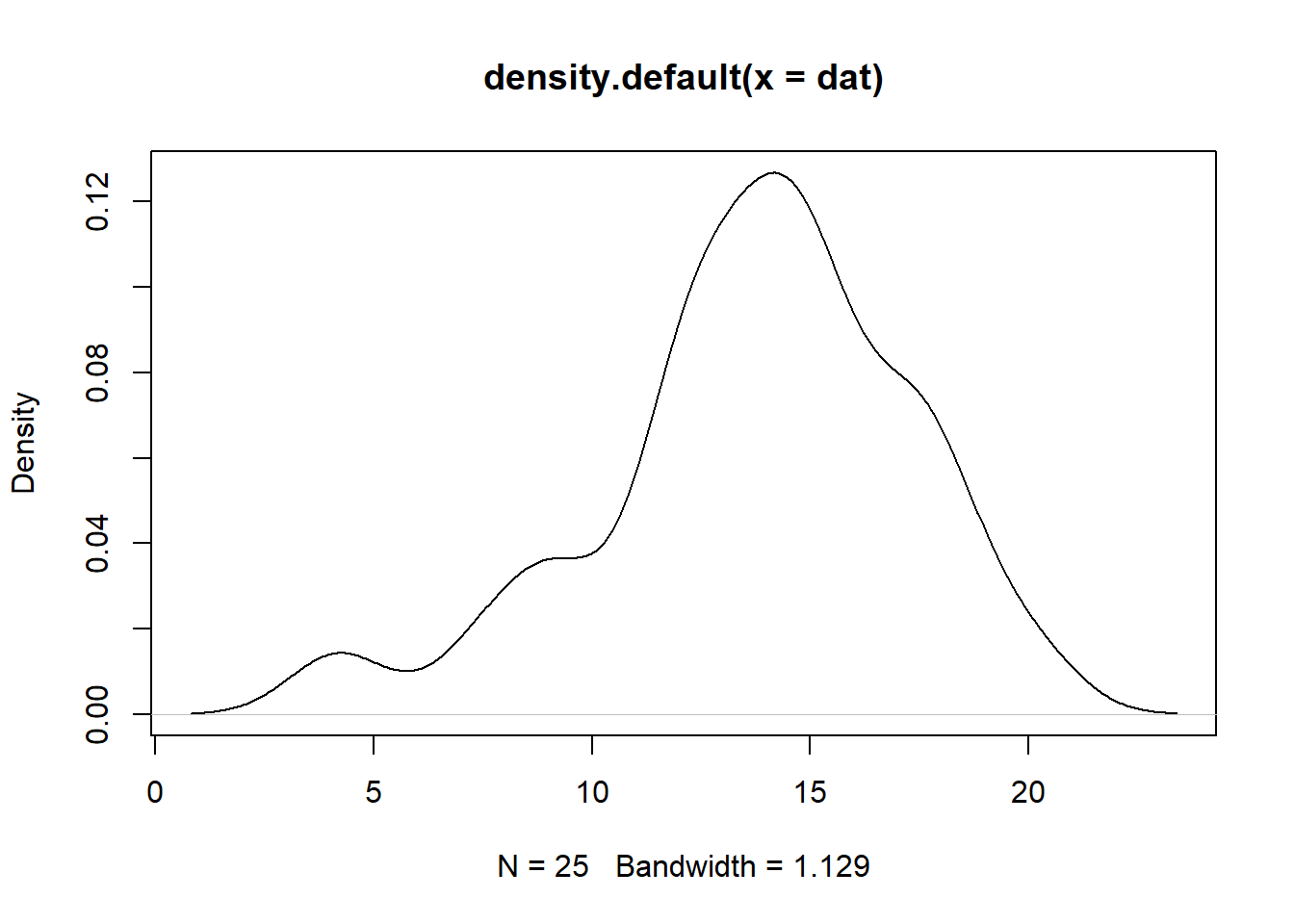
As we can see, the graph above does no exactly show a normal distribution however in this case we can run shapiro test to test for normality. This test confirms whether the normal distribution of the data is violated.
shapiro.test(dat)##
## Shapiro-Wilk normality test
##
## data: dat
## W = 0.96091, p-value = 0.4328Since p-value= 0.43 which is > 0.05, we conclude that the data distribution is not significantly different from normal distribution. However since sample size is less than 30, then one could argue that CI based on the \(t\) distribution would be the correct one.
Both functions are wrapped in a R package which you can download from github
install.packages("devtools")
library(devtools) # Make sure that the devtools library is loaded
install_github("firasfneish/CI-package")
library(CI)
To find more about the functions you could press F1 or use ?function_name like
?CI_t
?CI_z
Thanks to Prof. Michael Bach valuable comment, I have added this section, calculating CI based on Bootstrapping:
We can do lots of resampling and for each resampled data we calculate the mean and find difference between the sample data and the resampled one.
In the code below, 10000 resampled data are generated, their respective means are stored in vector “means”,then the difference between the sample mean and the vector means is taken and stored in a vector called “difference”. Only 20 values are shown for the sake of space!
Means = replicate( 10000, mean(sample(dat,length(dat),rep=T)) )
difference <- Means- mean(dat)
head(difference, 20)
## [1] 0.3992 0.0716 0.5148 -0.0356 -0.1932 1.0280 0.0188 -0.1592 -0.3472
## [10] 0.8116 0.8752 0.2824 0.8860 0.2216 -1.9352 1.5556 -0.1080 0.8600
## [19] 0.6432 -0.0728For calculating the 95% CI, we need the 97.5th and 2.5th percentiles from the vector “difference”
quantile(difference, c(.025, .975))## 2.5% 97.5%
## -1.43363 1.33725Now we can take the difference between the sample mean and the percentiles values above
mean(dat)- quantile(difference, c(.975, .025))## 97.5% 2.5%
## 12.38115 15.15203As before we see that at the 95% confidence level, the true mean of antibody titer production in the population is likely to be between 12.38 and 15.15.
Thank you for reading! If you have any question or suggestion then please feel free to comment below.